Multilayer Perceptron and Backpropagation

A single artificial neuron is not able to model real world problems and to achive realistic representations we must stack neurons in layers. The more neurons a layer have, the wider it is and the more layers a network has the deeper it is. Backpropagation is the algorithm that makes possible to adjust the weights from neurons in the early layers (front layers). Alongside Gradient Descent, backpropagation is one of the most important algorithms for artificial neural networks.

The Backpropagation is an old algorithm dated from 1970s but only in 1986 with the publishing of the paper "Learning Representations by Back-Propagating Errors" by Rumelhart, Hinton, and Williams that it was applied with neural networks. Although it is an old algorithm, backpropagation has being used in all deep learning models.

Geoffrey Hinton, on of the backpropagation creators, is an important figure in the machine learning community. He has been working with artificial neural networks for a long time and he was also one of the responsibles for the AlexNet network. Curiously, he is actively criticizing deep learning basic building blocks, precisely, the max pooling layer and the backpropagation algorithm. According to Hinton, the current models are not able to learn spatial hierarchies between simple and complex objects. One typical example is that we must provide images of the same object in many different angles, size and locations.

To make models learn similarly to what the human brain does in practice, Hinton and his team have introduced the capsules network. A capsule is a building block introduced to replace Convolutional kernels. And in order to train this network they also had to replace the backpropagation algorithm for another algorithm called dynamic routing between capsules. Initial experiments demonstrate that capsules network are more data efficient but they are is still slower than the usual Convolutional Neural Networks (CNN). Besides its computational requirements the capsules network need to be tested on different datasets and applications. Then, we will have a better idea if it can replace the CNNs. For a complete overview about the capsules network check this article.

To illustrate the Multilayer Perceptron (aka MLP) and the backpropagation, the figure below represents a MLP with 2 layers. The Layer 1 is the input layer and has 2 neurons and the Layer 0 is the output layer and has only one neuron. Any layer you add between the input and output layer is denominated as hidden layer.

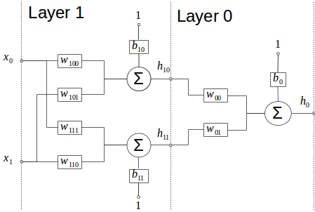
It is interesting to note that neurons in the same layer are not connected to each other. Also, each neuron is connected to all previous layer outputs (or inputs in the input layer case). Each deeplearning framework has a different naming convention for this scheme (layer): Pytorch calls it Linear layer; Caffe calls it Inner Product / Fully Connected Layer; Tensorflow calls it Dense layer.

The MLP network output is given by the perceptron definition and their interconnections inside the network. In our example the model equations are given by:

For each input \( (x_{0},x_{1}) \) there is a single \(h_{0}\) output. When these equations are evaluated this process is known as inference, prediction or forward pass/process.

Evaluating this model is a simple task, the real problem, that was a challenge to some scientists years ago was, how to (train) adjust the weights from the network front layers. That is when the backpropagation comes up.

To train a network (adjust the neurons weights) we use sets of input/output data \( (x_{0},x_{1}) \)/\( y \), an optimization algorithm (like the gradient descent) and a loss function (like the MSE). First, lets start with the MSE equation to compute the loss/error signal.

As we saw previously, we want to minimize the MSE function adjusting the MLP weights. We consider the input/output data constants and the network weights variables. We compute the partial derivative to every single weight we want to adjust.

The problem backpropagation solves is how to compute the output partial derivative to the weights \(\frac{∂h_{i}}{∂w}\). As the network becomes deeper it is almost impossible to manually compute this partial derivative. But since our example is simple we can compute them manually. For the last neuron we have:

From these equations we see the partial derivative depends on the input signal of each weight.

To compute the first layer weights we need to evaluate the output equation to the layer inputs \( (x_{0}, x_{1}) \).

Then we have:

Again we can see the partial derivative depends on the weight input signal, but now we have another term that comes from the last layer.

The backpropagation is an application of the derivative chain rule. Since the neurons from a layer \(f\) are only connected to neurons of a previous layer \(g\), we can see each layer as a function and the network as a function composition \( f(g) \). Therefore, to compute a partial derivative we have:

For example, we can decompose the \(\frac{∂h_{0}}{∂w_{100}} \) in two terms:

The whole equation becomes:

\(w_{00}\) does not have an index \([i]\) because it is a constant to the samples input.

The equation bellow is the loss signal backpropagated to the first neuron of layer 1.

Modern deeplearning frameworks store the differences \( (y[i] - h_{0}[i]) \) and backpropagate them layer per layer by multiplying the partial derivative to its inputs \( \frac{ ∂h_{out} }{ ∂h_{in}}\). These values are usually denominated as gradients. For each one of the neurons we have:

With the gradients we just need to multiply the weight input signal and compute the mean to obtain the \( \frac{∂}{∂w}MSE \)

The backpropagation is a simple algorithm to propagate the error signal to input layers. It is the main bottleneck to train deep neural networks because it requires a large amount of memory resources to store intermediate layer results and the gradients. The intermediate layer results may be stored after the forward pass or not. In case they are not stored in memory they will be computed during the backward pass which increases the training computation time. This relationship creates a memory/computation time trade-off to implement the backpropagation in graphics cards.

The backpropagation is very tricky and computing the partial derivatives can be a real challenge. In some cases it is very useful to decompose a layer in a graph where each node is a mathematical operation ( batch normalization example) .

A python script with the example above can be found at: repository.