Perceptron & Gradient Descent
The perceptron tries to mathematically represent a neuron but nowadays we know it is not realistic. The US-IARPA agency has even created a $100 million research program to reverse-engineer the algorithms of the brain. The Machine Intelligence from Cortical Networks (or MICrONS) seeks to revolutionize machine learning with more truthful algorithms.
Neural networks are built with a combination of several perceptrons (and much more). To completely understand neural networks it is important to study the perceptron and understand what they represent.
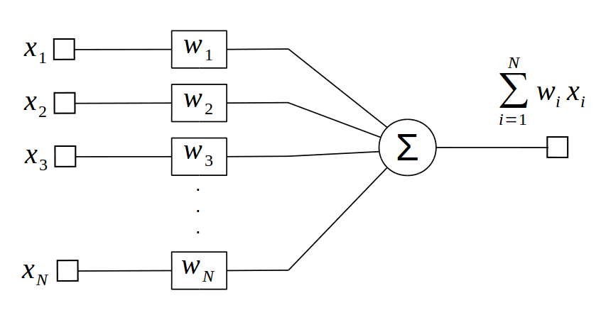
The perceptron is defined according to the following function: $$ f(x) = \sum_{i=1}^{N} { w_{i} x_{i} } $$ $$ f(x) = w_{1} x_{1} + w_{2} x_{2} + ... + w_{N} x_{N} $$ It represents the summation of \(N\) inputs \(x\) multiplied by \(N\) weights \(w\). The perceptron is usualy represented by the block diagram below.
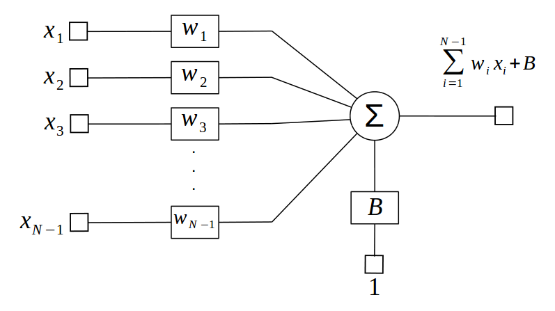
It can also be represented with a bias when one of its input is equal to one. It is just important to note that the bias is a weight like any other.
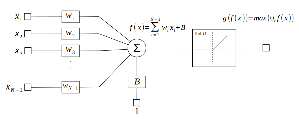
The perceptron is usually followed by an activation funtion that adds non-linearity to the whole model. Real world problems are non-linear and almost all deep neural networks make use of activation funtions. A common activation function is the ReLU, short for Rectified Linear Unit, which zeroes negative outputs from the perceptron. $$ g(f(x)) = max(0,f(x)) $$
But how is this model useful? The trick is that we can adjust the weights to match specific outputs, process denominated as training process. How these weights are adjusted depend on loss functions also known as loss, target or error functions. To illustrate how the weights are adjusted lets create a toy problem for linear regression.
In this case we are not making use of activation functions.
Imagine we have a perceptron with one input and bias. Its equation is reduced to:
$$ f(x) = { w x + b } $$This equation can represent any line in a \( (f, x) \) cartesian coordinate system but we want to adjust this function to a set of points. In other words, we need to find the weights \( w, b \) that fit the data.
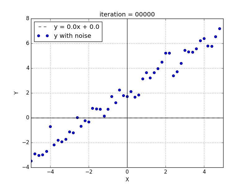
We can generate a set of data with normal distribution around a line. The blue dots from the figure below represents points around the line \(y = 1x + 2 \). The normal distribution has zero mean and 0.5 standard deviation.
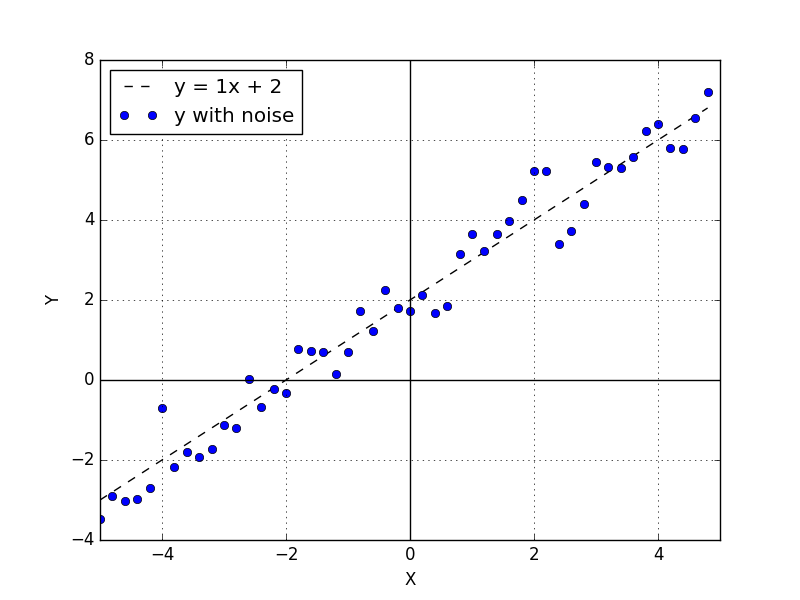
If we use the perceptron to fit to this data we have to find weights equal to \(w = 1\) and \(b = 2\). In this particular toy problem we are aware of these values but in real world problems we don't know the function that is hidden under the noise.
Before we start adjusting the perceptron weights we need to select a loss function. The loss funtion is also called error function or target function. For regression problems a very common function is the Mean Squared Error (MSE).
$$ MSE = \frac{1}{N} \sum_{i=1}^{N} { (d_{i} - h_{i})^2 } $$The MSE is computed with the differences between the data and a hypothesis function \(h\). This differences or distances are errors between your data and the hypothesis. In out case the hypothesis function is the one input perceptron function, but \(h\) could be any function.
When we use the MSE we want to minimize the summation of the distances between the data and the hypothesis. In other words we want to find a local minimum.
For the perceptron we want to adjust the neuron weights that minimize the MSE. We consider each perceptron weights an independent variable and we compute the derivative of the MSE regarding the weights. It is interesting to keep in mind that the loss function variables are the network weights not the network inputs.
$$ h(x) = { w x + b } $$ $$ \frac{∂}{∂w}MSE = - \frac{2}{N} \sum_{i=1}^{N} { (d_{i} - h_{i}) * x_{i} } $$ $$ \frac{∂}{∂b}MSE = - \frac{2}{N} \sum_{i=1}^{N} { (d_{i} - h_{i}) } $$We adjust the weights with these derivatives and an update equation. The update equation idea is to use the derivatives to adjust the weights towards the direction that minimizes the error function.
$$ w = w - lr * \frac{∂}{∂w}MSE $$ $$ b = b - lr * \frac{∂}{∂b}MSE $$\(lr\) is the learning rate, a small factor used to reduce the devirative value. This process is repeated several times. Each update is called an iteration and after a number of iterations we stop this process. \(lr\) and the number of iterations are called hyperparameters and there is no rationale to define these variables.
We set the weights initial values to 0 and with this dataset, a \(lr = 0.01\) and a number of iterations \(= 300\) the final perceptron weights are \(w = 1.03\) and \(b = 1.98\).
A python script with examples can be found at: repository.